Table of Contents
[ misc ][ cdo ][ journals ][ fortran ][ mpi ][ paper notes ][ Beamte ]
Misc
This is a page for various notes and quick tests …
Many times I had someone on the other part of the line and
wanted to talk about mathematics ... so you need some space
where you can quickly type some ideas in LaTeX and the other
person with internet connection can read it ...
Da Redesign 1
$a$: all information on bonds, spots or collections or records of observations
$dim_a$: dimension of bonds
$y$: Observation vector, List of observation values
$dim_y$: dimenension of obs
$is$: Ispace, Interpolation space, list of interpolation points and variables
$dim_i$: dimension of interpolation space
$y-i-list$: values needed for y from $is$, this is a vector of some dimension $dim_{yi}$, referenced by vectors yii and yil of integers, where yii(jy) is the starting index and yil(jy) is the number of points needed for the observation with index jy.
Da Redesign 2
Maths Notation
Linearisierung $$ f(x) = f(x_0) + df*(x-x_0), \hspace{1cm} q_i(t,q) = q_i(t_0,q_0) + \frac{dq_i}{dt} (t-t_0) + \frac{dq_i}{dq} (q-q_0) $$
$$
A = \left( \begin{array}{cc}
1 & 0
0 & 1
v_1 & v_2
\end{array} \right), \hspace{1cm}
A^{T} = \left( \begin{array}{cc}
1 & 0 & v_1
0 & 1 & v_2
\end{array} \right)
$$
$$
x = \left( \begin{array}{c} t
q \end{array}\right), \hspace{1cm}
A * x = \left( \begin{array}{c} t
q
q_i \end{array} \right)
$$
$z$ be the reflectance using $H_{s}$ MFASIS, then:
$$
H_{s} = (\alpha_1, \alpha_2, \alpha_3),
\hspace{1cm} \left( \begin{array}{c} t
q
q_i \end{array} \right) =
\left( \begin{array}{c} \alpha_1 z
\alpha_2 z
\alpha_3 z \end{array} \right) = H_s^T z
$$
$$
A^T H^T z = A^T \left( \begin{array}{c} \alpha_1 z
\alpha_2 z
\alpha_3 z \end{array} \right)
= \left( \begin{array}{c} (\alpha_1 + v_1 \alpha_3 ) z
(\alpha_2 + v_2 \alpha_3 ) z
\end{array} \right) \hspace{1cm}
H_s * A = \left( \begin{array}{cc} (\alpha_1 + v_1 \alpha_3 ) & (\alpha_2 + v_2 \alpha_3 )
\end{array} \right)
$$
Maths Notation
$$ \frac{dx'}{dt}(\rho,t)\Big|_{t=0} = 0 \hspace{3cm} (3.4) $$
Talk Data Assimilation
A general introductory talk into data assimilation for numerical weather prediction: http://scienceatlas.com/potthast/_media/talk_potthast_reading_2014_11.pdf and http://scienceatlas.com/potthast/_media/potthast_icon_bacy_tour.pdf
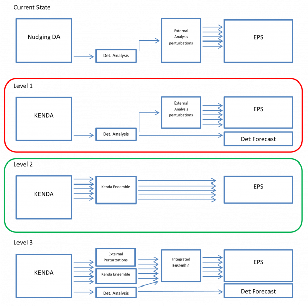
KENDA Concept
Approximations in Fourier Space
Aamir August 30. We try to approximate given function values $$ f(x_1), f(x_2), f(x_3), …, f(x_m) $$ by a function of the form \begin{equation} g(x) = \sum_{\ell=-L}^{L} g_{\ell} e^{i \ell x}, \;\; x \in [0, 2\pi]. \end{equation} We do it
- globally with large $L$,
- globally with small $L$ (i.e. low modes)
- locally with small $L$, this is called \\Localization\\.
SEVIRI Testing
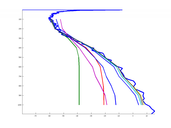
The following graphics shows some testing with RTTOV 10 and SEVIRI Radiances. The blue profile is the demo temperature profile provided by RTTOV. The other lines show the brightness temperature (BT) of SEVIRI (in degrees Celsius) given by the channels when an opaque cloud is put into the different heights (in hPa) shown on the left.
Test PHP
Embedding PHP works, writing “test” via php: <php> echo “test”; </php>
Natalie June 10, 2013
I) Theory for the Stability of Classification in General
… we investigated the stability of image classes under the influence of the above compact operator $A$. Our main results show that
- the image classes of two stably separable linear classes will not be stably separable if the normal vector to the separating hyperplane is not in the range of the adjoint operator $A^{\ast}$.
- For sequences of uniformly stably separable linear classes, the stability of the separation is not preserved when we map them into the image space.
- For two elliptical classes, in any case the image classes remain stably separable.
We note that the second point has consequences for non-linear classes as well, since in the smooth case they are made up of sequences of linear classes. If the nonlinear class has a sequence of normal vectors which span an infinite dimensional subspace, then the nonlinear image classes cannot be stably separable.
II) Investigate the Stability of Key Algorithms
We have investigated two well-known algorithms for classification: the FLD as a key method for supervised classification and the K-Means Algorithm combined with a PCA as a well established approach to unsupervised classfication.
- For FLD, by tools of numerical analysis we have proven that - applied to image data - the classes inherit the ill-posedness of the mapping $A$.
III) Investigate the Stability of Classifications in Magnetic Tomography (in particular for Fuel Cells)
In Chapter 3, we presented a concise investigation of the ill-posedness of classifications for magnetic tomography, with a particular emphasis on classifications for fuel-cells as an important application area.
Natalie June 6, 2013
Hello 
Statement: Let $A: X \rightarrow Y$ be a compact operator and $X$ be infinite dimensional. Then there is a sequence $\varphi_n \in X$ with $||\varphi_n||=1$ such that \begin{equation} A\varphi_n \rightarrow 0, \;\; n\rightarrow \infty. \end{equation}
$\newcommand{\tvarphi}{\tilde{\varphi}} \newcommand{\tpsi}{\tilde{\psi}}$ $Proof.$ Since $A^{-1}$ is unbounded, this means that there exists a sequence $\tpsi_n \in Y$ with norm $||\tpsi_n || = 1$ and \begin{equation}
| A | {-1}\tpsi_n | |
|---|---|---|
\end{equation} We define \begin{equation} \varphi_n := \frac{A^{-1} \tpsi_n}{||A^{-1}\tpsi_n||}, \;\; n \in \mathbb{N}. \end{equation} Then we have $$
| A \varphi_n | = \frac{ | \tpsi_n | }{ | A | {-1}\tpsi_n | |||||
|---|---|---|---|---|---|---|---|---|---|---|
$$ and the proof is complete $\Box$.
Mathematical Notation Discussion
Use $x$ for points in $\mathbb{R}^3$, then \begin{equation} \Omega = \Big\{ x \in \bigcup_{i=1}^{K} C_i \Big\} \end{equation}
probably better to write \begin{equation} \Omega = \bigcup_{C \in \cal{C}} C \end{equation} where \begin{equation} \cal{C} = \Big\{ L_{j} …\Big\} \end{equation}
Consider a simple situation like
| $x_1$ | $x_2$ |
| $x_3$ | $x_4$ |
and now two slants, given by
\begin{eqnarray}
s_1 & = & x_1 + x_4
s_2 & = & x_2 + x_4
\end{eqnarray}
leading to a matrix equation
\begin{equation}
\left( \begin{array}{ccc}
1 & 0 & 0 & 1
0 & 1 & 0 & 1
\end{array} \right) \circ
\left( \begin{array}{c}
x_1
x_2
x_3
x_4
\end{array} \right)
= \left( \begin{array}{c}
s_1
s_2
\end{array} \right)
\end{equation}
We might include some weighting function for taking care of the lenght of
the path of the ray through the area denoted by $x_j$, $j=1,…,4$, then we obtain
a weighted system of the form
\begin{eqnarray}
s_1 & = & w_{1,1} x_1 + w_{1,4} x_4
s_2 & = & w_{2,2} x_2 + w_{2,4} x_4
\end{eqnarray}
A ray starting at $b \in \mathbb{R}^3$ with direction $\nu \in \mathbb{R}^3$ is given by \begin{equation} L = \{ x = b + \eta \cdot \nu| \; \eta > 0 \}. \end{equation} An integral along $L$ is written as \begin{equation} f(b,\nu) := \int_{L} \varphi(y) ds(y), \end{equation} where $ds(y)$ denotes the standard Eucliedean measure along $L$. Alternatively, when $||\nu|| = 1$, you might write \begin{equation} f(b,\nu) = \int_{0}^{\infty} \varphi(b + \eta \nu) d\eta \end{equation} We use the notation \begin{equation} (R\varphi)(b,\nu) := f(b,\nu), \;\; b \in \mathcal{B}, \; \nu \in \mathcal{N} \end{equation} where $\mathcal{B}$ and $\mathcal{N}$ denote the set of our base stations and the set of slant directions measured by the stations over some time interval. In discretized form, the operator ${\bf H}$ maps $\vec{\varphi} \in \mathbb{R}^n$ into $\vec{f} \in \mathbb{R}^m$. It is a linear operator and, thus, we obtain a matrix operator from $\mathbb{R}^n$ into $\mathbb{R}^m$. Thus, GPS tomography boiles down to solving a linear finite dimensional system \begin{equation} {\bf H} \vec{\varphi} = \vec{f} \end{equation} We solve it by 3dVar or Tikhonov Regularization, respectively, which is \begin{equation} \varphi^{(a)} = \varphi^{(b)} + B H^{T}( R + H B H^{T})^{-1}( f - H \varphi^{(b)} ), \end{equation} which is minimizing \begin{equation} J(\varphi) = ||\varphi - \varphi^{(b)}||^2_{B^{-1}} + ||f - H \varphi||^{2}_{R^{-1}}. \end{equation} Adaptive regularization would change the regularization term \begin{equation} ||\varphi - \varphi^{(b)}||^2_{B^{-1}} \end{equation}
Natalie 24.4.2013
We first select a subsequence of $\mathbb{N}$ such that a point in the support $\chi_i$ of $v_{k_{i}}$ has limiting point $x_{\ast} \in \Omega$. This is possible since any bounded sequence in $\mathbb{R}$ has a convergent subsequence. We call it $k_{i}$ again.
Given $\epsilon>0$ there is $i>0$ such that $$
| v_{k_{i}} - v_{\ast} |
$$ So we know that on the exterior of the support $\Omega_{k_{i}}$ of $v_{k_{i}}$ we have $$
| v_{\ast} | _{L | |
$$ For a function $v_{\ast} \in L^2(\Omega)$ we have that \begin{eqnarray}
| \int_{\Omega_{k_{i}}} | v_{\ast}(y) | 2 dy | |
|---|---|---|---|
\end{eqnarray} Now, we obtain \begin{eqnarray}
| v_{\ast} | _{L | 2(\Omega)} | {2} & = & | v_{\ast} | _{L | 2(\Omega \setminus \Omega_{k_{i}})} | |||
|---|---|---|---|---|---|---|---|---|---|
+ ||v_{\ast}||_{L^2(\Omega_{k_{i}})}^2
\nonumber
& \rightarrow & 0, \;\; i \rightarrow \infty.
\end{eqnarray}
Natalie 9.5.2013
Simple question: is $\frac{1}{x-y}$ analytic in $x$ for fixed $y$?
Answer 1) Yes, since the sum and product of analytic functions are analytic, and the quotient of analytic functions are analytic where the denominator is non-zero.
Answer 2) We use the series expansion $$ \frac{1}{x-y} = (-1) \sum_{n=1}^{\infty} \frac{x^n}{y^{n+1}} $$ for $|x|<|y|$, which I took from Wolfram. For $|x|<\rho \cdot |y|$ with $\rho<1$ we have $$
| \frac{x | n}{y | {n+1}} | < \frac{1}{y} \rho |
|---|
$$ such that $$
| \sum_{n=1} | {\infty} \frac{x | n}{y | {n+1}} | < \frac{1}{ | y | } \sum_{n=1} | {\infty} \rho |
|---|
$$ is absolutely convergent by the geometric series. Thus, $\frac{1}{x-y}$ is analytic on $|x|<|y|$. For $|x|>|y|$ we use $$ \frac{1}{x-y} = \sum_{n=1}^{\infty} \frac{y^n}{x^{n+1}} $$ analogously.
little statement
Let $g$ be a function in $L^2(\Omega)$ and let $\Omega_i$ be subsets of $\Omega$ with $|\Omega_i| \rightarrow 0$ for $i \rightarrow \infty$. Then we have \begin{equation} \label{eq1} \int_{\Omega_i} |g|^2 dy \rightarrow 0, \;\; i \rightarrow \infty. \end{equation}
Proof. Given $\epsilon$ there is a bounded function $f \in C^{\infty}(\Omega)$ such that \begin{equation} \label{eq2}
| g -f | _{L | 2(\Omega)} | |
|---|---|---|---|
\end{equation}
Further, for a function $f \in C^{\infty}(\Omega)$ given $\epsilon$
we find $i_0>0$ such that
\begin{equation}
\label{eq3}
\int_{\Omega_{i}} |f(y)|^2 dy \leq \frac{\epsilon}{4}
\end{equation}
for all $i\geq i_0$. Now, given $\epsilon$ we first choose $f \in C^{\infty}$ such that
(\ref{eq2}) is satisfied. Then, we choose $i_0$ such that (\ref{eq3}) is true. This
yields
\begin{eqnarray}
\int_{\Omega_i} |g|^2 dy & = & \int_{\Omega_i} |g-f + f|^2 dy
& \leq & 2 (\int_{\Omega_i} |g-f|^2 dy + \int_{\Omega_i} |f|^2 dy )
& \leq & 2(\frac{\epsilon}{4} + \frac{\epsilon}{4}) = \epsilon
\end{eqnarray}
for $i \geq i_0$.
$\Box$
another statement
$A: X \rightarrow Y$ compact, $\varphi_n$ bounded sequence in $X$, then $\psi_n := A\varphi_n$ has a convergent subsequence, which we relable to use index $n$ again.
$\psi_n \rightarrow \psi_{\ast} \in Y$. If $\psi_{\ast} \in R(A)$, then there exists $\varphi_{\ast} \in X$ such that $A \varphi_{\ast} = \psi_{\ast}$. Defining $\tilde{\varphi}_{n}:= \varphi_n - \varphi_{\ast}$ we obtain a sequence such that $$ A \tilde{\varphi}_{n} \rightarrow 0, \;\; n \rightarrow \infty. $$
another statement
\begin{eqnarray}
\tilde{Y}^{T} \tilde{R}^{-1} \tilde{Y} & = & Y^{T} A^{T} (A R A^{T})^{-1} A Y \nonumber
& = & Y^{T} A^{T} (A^{T})^{-1} R^{-1} A^{-1} A Y \nonumber
& = & Y^{T} R^{-1} Y
\end{eqnarray}
Which metric to use?
$$ D{y} := \frac{y_{2}-y_{1}}{h} $$
in other words
$$
{\bf y} := \left( \begin{array}{c}
y_{1}
D{y}
\end{array} \right)
$$
and
$$
\| {\bf y} - {\bf y^{(o)}} \|^2 := \| y_{1} - y_{1}^{(o)} \|^2 + \| D{y} - D{y}^{(o)} \|^2
$$
or the original one
\begin{eqnarray}
\| {\bf y} - {\bf y^{(o)}} \|^2 & := & \| {\bf y} - {\bf y^{(o)}} \|_{\tilde{R}}^2 \nonumber
& = &
({\bf y} - {\bf y^{(o)}})^{T} (A^{T})^{-1} R^{-1} A^{-1} ({\bf y} - {\bf y^{(o)}})
\end{eqnarray}
$$
A = \left( \begin{array}{cc}
1 & 0
-\frac{1}{h} & \frac{1}{h}
\end{array}\right)
$$


